1. The Integrated Prediction Pipeline - T3SEpp

1.1. The Frame of T3SEpp

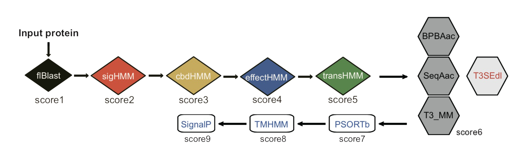
A typical T3SE protein should show the following property: (1) containing a putative T3S signal sequence (Module 1a - sigHMM) or showing the signal sequence features (Module 1b - T3SEppML); (2) showing full-length sequence homology (Module 2a - flBlast) with known T3SE families or containing a conserved effector domain (Module 2b - effectHMM); (3) having a conserved motif in the chaperone-binding domain (Module 3 - cbdHMM); (4) containing a putative T3SE regulatory motif within the gene promoter region (Module 4 - transHMM); (5) being not a cytoplasmic protein (Module 5 - PSORTb), without a putative signal peptide (Module 6 - SignalP) and not a trans-membrane protein (Module 7 - TMHMM). T3SEpp integrated the above feature prediction results with the modules indicated. A linear model was adopted to connect the results of different modules. The modules newly developed were in italic and blue font while those cited from other groups were shown in red.

1.2. Optimized Hyperparameters and Performance of T3SEpp

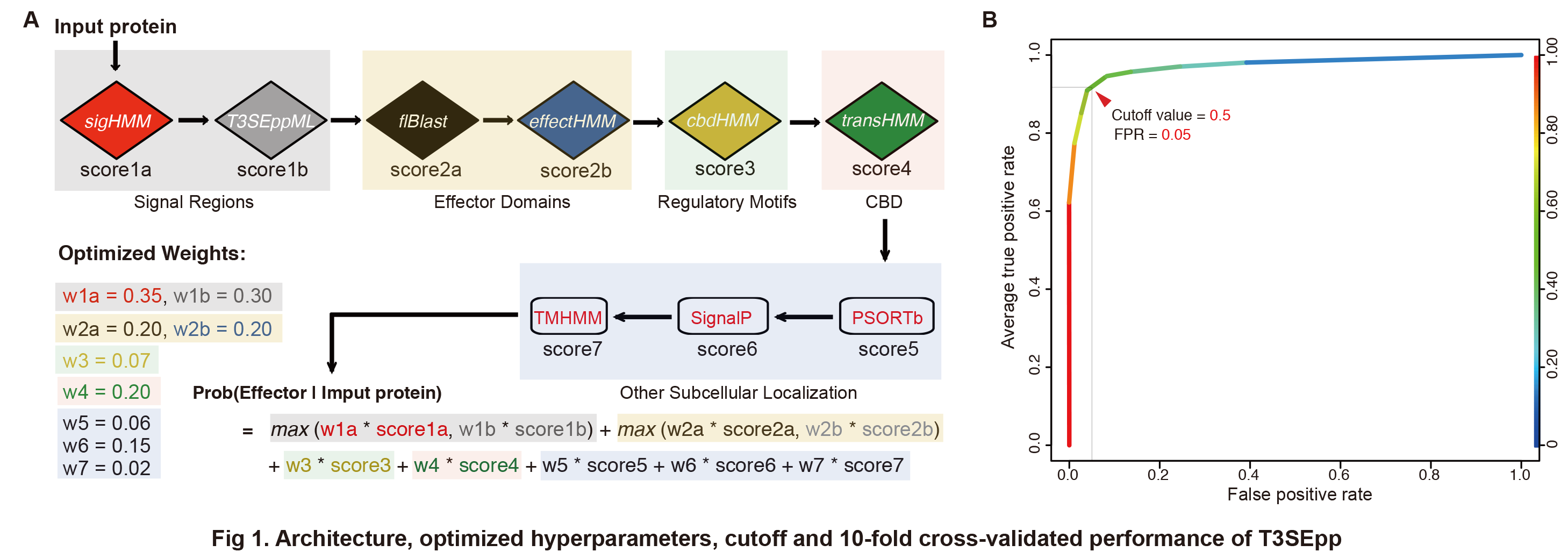
A 10-fold cross-validation strategy was used to optimize the hyperparameters of T3SEpp, i.e., the weight of each module. The T3SEpp architecture and optimized weights were shown in Fig 1A. The 10-fold cross-validated AUC of the ROC curves of the training datasets for the models with optimized parameters reached 0.976 (Fig 1B). According to the average ROC curve, a cutoff, 0.5, was selected and used as the default prediction cutoff value for web-based or standalone T3SEpp, to compromise both the specificity and sensitivity (Fig 1B).

2. Module 1a: Prediction of Conserved T3S Signals – sigHMM

2.1. T3S Signal Scanning

The N-terminal sequences of T3SEs have been considered with putative signals guiding specific type III secretion. However, the signals are atypical and difficult to detect. The Module 1 contains two sub-modules to screen the T3S signals, namely sigHMM and T3SEppML, respectively. sigHMM was designed to detect the conserved T3S signal peptide families within the N-terminal fragments of proteins to be analyzed. In contrast, T3SEppML was an ensemble model comprising six machine-learning sub-models, which predicted the possibly atypical T3S signal features from the N-terminal fragments of candidate proteins.

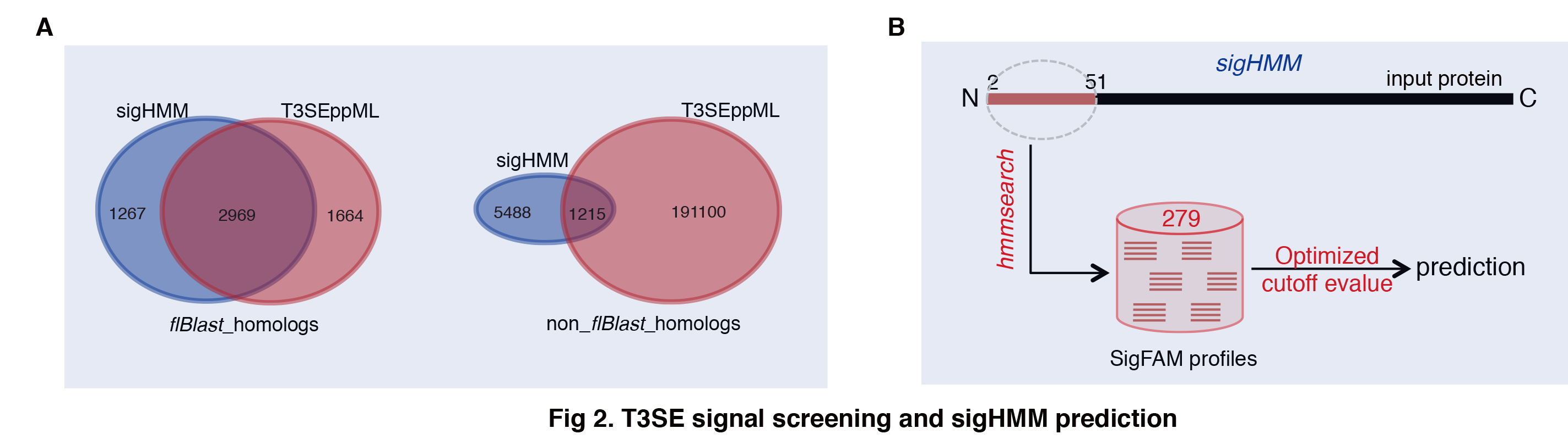
The sigHMM hits were not necessarily captured by T3SEppML, vice versa. In T3SEpp, to control the false positive rate of T3SEppML, we leveled up the specificity, and therefore, the overlap between the hits of sigHMM and T3SEppML turned smaller (Fig 2A). Therefore, the two sub-modules have complement effect for each other. While sigHMM hits could have a higher likelihood to be a true T3SE since the signals are more typical, T3SEppML could provide more relatively novel T3SE candidates that exhibited the atypical T3S signal features. In T3SEppML pipeline, a larger weight was assigned to sigHMM (0.35) than to T3SEppML (0.30), but both showed the largest contribution to the overall prediction.

2.2. Methodology of sigHMM

The framework of sigHMM prediction was shown in Fig 2B and summarized briefly as below.

    (1) Family clustering. 519 manually annotated, validated T3SEs were retrieved from T3Enc (v201703). The N-terminal 50-aa peptide fragments were extracted from effectors after starting ‘M’s were removed. JAligner was adopted to implement the Smith-Waterman algorithm, making all vs. all pairwise alignment. A pair of signal peptide fragments was considered with homology for a minimum cutoff of 30% identity for 70% length of both the aligned peptide fragments. The signal sequences were grouped into clusters using an iterative homolog-networking algorithm. No homology (defined similarly) was detected between members from any two different clusters. Clustalw was used to make multiple sequence alignment for the signal peptide fragments from each cluster with the default parameters. A cluster could be further separated into different families among which no homologous blocks were detected. In total, the signal sequences were clustered into 379 signal families.

    (2) Family profiles. The signal peptide fragments from each signal family were retrieved for building the family profile. For the singleton family, all orthologs of the effector were retrieved from the bacterial strains of the same genus. The N-terminal 50-aa peptides were extracted and the non-identical but homologous (>=70% identity for full length) fragments were retained as the family members based on all vs. all pairwise alignment results. HMMER 3.1 was used to build the family profiles. For each family, the fragment sequences of the members were aligned with hmmalign and used to build the Hidden Markov Model (HMM) profile with hmmbuild. In total, we built the profiles for 279 signal families, which were curated in sigHMM module of the T3SEpp package.

    (3) Similarity cutoffs. The verified members of each family were aligned against the corresponding family profile with the HMMER module hmmsearch, and the minimum similarity level was recorded (E-value) and used as the prediction cutoff.

    (4) Prediction. For any candidate protein, its N-terminal 50-aa fragment is extracted (without the starting ‘M’) and searched for the possible conserved signal sequences by alignment against the profile of each signal family, using hmmsearch with the similarity cutoff determined as described above. A program sigHMM was developed to implement the prediction automatically.

3. Module 1b: Prediction of Atypical T3S Signals – T3SEppML

3.1. The Frame and Performance of T3SEppML

T3SEppML is an ensemble module comprising six machine-learning models. All the models predict the atypical amino acid composition features learned from signal regions of known T3SEs, i.e., N-terminal 100-aa peptide fragments. The six models include BPBAac, BPBent, T3_MM, SeqAac, T3SEdnn and T3SErnn (Fig 3A). A voting approach was adopted to integrate the prediction results from each of the models. 10-fold cross-validation assessment suggested that the integration of the models improved the prediction performance dramatically, mainly by increasing the TPR but reduce the FPR. T3SEppML reached an average AUC of 0.96, and the average ROC curve indicated an inflection point at 0.5 (3/6 positive), which showed best compromise between FPR (~10%) and sensitivity (~90%) and therefore used as the cutoff for prediction (Fig 3B).

3.2. T3SEppML-sp*

The number varied a lot for T3SEs identified from different groups of T3SSs or bacterial genera, and therefore it remains difficult to train machine-learning models specifically predicting the effectors from each T3SS group or bacterial genus / species. However, it is feasible for some subset of the T3SS groups and bacterial genera, adopting algorithms relatively insensitive to data size, e.g., T3_MM. Currently, we have trained specific T3_MM, BPBAac, BPBent and SeqAac models for animal and plant microbes, Cluster I~VII and X T3SSs, and bacterial genera including Yersinia, Salmonella, Vibrio, Chlamydia, Escherichia, Shigella, Pseudomonas, Xanthomonas, Ralstonia and Burkholderia. However, the ensemble module, T3SEppML-sp*, has not yet been confirmed for the better performance, but users are encouraged to contact us to obtain and test it.

3.3. BPBAac

The current version of BPBAac (2.0) was not different from the original version as for the algorithms (Wang et al., 2011, Bioinformatics, 27:777-84), but was retrained with updated training datasets and optimized for the SVM kernels and related parameters.

    (1) Methodology. BPBAac calculated the position-specific composition of each species of amino acid at each position of the N-terminal 100-aa fragments for both positive and negative datasets to get the two position-specific Aac profiles, followed by representing each training or interesting 100-aa peptide with the bi-profile Aac in a vector with 200 elements. The feature matrix was used for training SVM models or prediction with the optimized SVM models. Four SVM kernels and corresponding parameters were all optimized with a 10-fold cross-validation grid search strategy.

     (2) Optimized parameters and performance. BPBAac adopted a ‘linear’ kernel and an optimized cost of 0.0039. The average AUC of 10-fold cross-validated ROC curves reached 0.824 (Fig 3C).

   (3) Prediction. N-terminal 100-aa peptides of candidate proteins were detected for possible T3S signals with BPBAac. The version of BPBAac was integrated in T3SEppML. However, it could also be implemented independently. A cutoff, 0, was selected to predict the candidate sequence to be with or without T3S signals. At this cutoff, the sensitivity was ~72% at an FPR of ~20%.

3.4. BPBent

BPBent was built for the first time for T3SE prediction.

    (1) Methodology. Similar to BPBAac, but instead of position-specific Aac, BPBent calculated the individual relative entropy for position-specific Aac between T3S signal sequences and total bacterial proteins, between non-T3S sequences and total bacterial proteins, and between T3S signal sequences and non-T3S sequences, respectively. The tri-profile relative entropy values were represented as a vector for each sequence, and the feature matrixes were trained with SVM models as done for BPBAac. The kernel selection and parameter optimization were also similar to the procedure for BPBAac as described above.

     (2) Optimized parameters and performance. BPBent adopted a ‘RBF’ kernel and optimized gamma of 0.0039 and cost of 0.5. The average AUC of 10-fold cross-validated ROC curves reached 0.818 (Fig 3C).

    (3) Prediction. N-terminal 100-aa peptides of candidate proteins were detected for possible T3S signals with BPBent. The version of BPBent was integrated in T3SEppML. However, it could also be implemented independently. A cutoff, 0, was selected to predict the candidate sequence to be with or without T3S signals. At this cutoff, the sensitivity was ~71% at an FPR of ~22%.

3.5. T3_MM

The current version of T3_MM (2.0) was not different from the original version as for the algorithms (Wang et al., 2013, PLoS One, 8:e58173), but was retrained with updated training datasets.

    (1) Methodology. T3_MM calculated the probabilities of any species of amino acids conditional on the amino acid composition in its adjacently preceding position for both positive and negative N-terminal 100-aa training sequences. For each sequence, two Markov chains were built with each amino acid represented with the conditional probability values extracted from positive and negative training dataset respectively, followed by calculation of the logarithum likelihood ratio (positive/negative), which was used for eventual classification.

     (2) Optimized parameters and performance. The performance of T3_MM depends on the training datasets rather than parameters. The average AUC of 10-fold cross-validated ROC curves reached 0.907 (Fig 3D).

    (3) Prediction. N-terminal 100-aa peptides of candidate proteins were detected for possible T3S signals with T3_MM. The version of T3_MM was integrated in T3SEppML. However, it could also be implemented independently. A cutoff, 0, was selected to predict the candidate sequence to be with or without T3S signals. At this cutoff, the sensitivity was ~78% at an FPR of ~8%.

3.6. SeqAac

SeqAac was also developed for the first time. Different from BPBAac, BPBent and T3_MM, SeqAac learned comprehensive sequential features of T3S signal peptide fragments.

    (1) Methodology. In total, 431 sequential features were observed and compared between T3S and non-T3S sequences, including composition of individual amino acids (20), bi-residues (20x20 = 400) and amino acids of 11 specific properties (aliphatic, aromatic, hydrophobic, alcohol, polar, tiny, small, bulky, positively charged, negatively charged and charged). Bonferroni-corrected Students’ t-tests were performed between the sequential composition of features between T3S and non-T3S sequences, and the top 30 features were selected for model training. For each sequence, the composition of each feature was calculated and put into a vector. The matrix composed by the 30-feature vectors for each training dataset was used for a decision tree building and pruning with the R ‘rpart’ package.

     (2) Optimized parameters and performance. The tree architecture, features and their decision cutoffs were shown in Fig 3E. The average accuracy of SeqAac was 0.758.

    (3) Prediction. N-terminal 100-aa peptides of candidate proteins were detected for possible T3S signals with SeqAac. The version of SeqAac was integrated in T3SEppML. However, it could also be implemented independently. SeqAac made decision independent on an eventual cutoff. The sensitivity was ~76% at an estimated FPR of ~24%.

3.7. T3SEdl

Two deep-learning models were also trained to learn the hierarchical Aac features buried in T3S signal sequences, namely T3SEdnn and T3SErnn. Both models were integrated in a sub-module, T3SEdl, the latter of which was further integrated in T3SEppML.

      T3SErnn was comprised of convolution layers, recurrent layers and fully connected dense layers. The input was a 100 x 20 matrix, where 100 was the length of sequence and 20 was the size of amino acid vocabulary. The convolutional neural network extracted motif information using 30 filters with different sizes (5 for each of the sizes 1, 3, 5, 7, 9, 11). By concatenating the above features, we obtained a 120 x 5 feature map. Then we applied another convolution layer with 50 filters of size 3 x 120 to this feature map and obtained a 120 x 50 feature map as input to the recurrent layer. The recurrent neural network scanned the above feature map using 256 LSTM units in two directions and returned the last output in the output sequence. Finally, the concatenation of the outputs of the recurrent neural network was used as input to a fully connected dense layer with 512 units and output the final prediction score. The parameters were optimized using Adaptive Moment Estimation (Adam) with cross entropy as the loss function.

      The T3SEdnn model was composed of three components, i.e., the input layer, the hidden layers and the output layer. The input of the model was the stretch of a 100 x 20 one-hot matrix. Then the model projected the input feature into new spaces layer-by-layer. In particular, the model included five hidden layers with 1024, 512, 256, 128 and 10 units respectively. The output layer of the model was a logistic repression classifier with a sigmoid function as activation function. The parameters were optimized using Root Mean Square Propagation (RMSProp) with cross entropy as the loss function.

      10-fold cross-validation performance assessment of the T3SErnn and T3SEdnn disclosed an average AUC of 0.89 and 0.86, respectively, superior to that of ANN and SVM models (Fig 3F). N-terminal 100-aa peptides of candidate proteins were detected for possible T3S signals with both T3SErnn and T3SEdnn. The T3SEdl was both integrated in T3SEppML and released independently. Both models made decision independent on a cutoff of 0.5. T3SErnn and T3SEdnn showed a sensitivity of ~80% and ~77% at an FPR of ~12% and ~14%, respectively.

4. Module 2a: Prediction of Homologs of Validated Effectors – flBlast

A T3SE could have a conserved T3S signal sequence or atypical T3S signal features but contains a novel effector domain. Similarly, a T3SE could also have a conserved domain of known T3SE families but does not show similarity to putative T3S signal sequences due to the presence of a novel signal sequence. Some proteins could show overall similarity to the known T3SEs but no apparent conservation in either signal or effector regions. To find out the global and fragmental homologs of known effectors, we developed flBlast, sigHMM and effectHMM (Guo et al., 2018, Curr Bioinf, 13:280-289). One of the models, sigHMM, was introduced previously, while flBlast and ffectHMM were placed together in a single module of T3SEpp, since they mainly measured the conservation of effector domains.

4.1. Methodology of flBlast

The flBlast mainly used BLASTp to make the sequence alignment between candidate proteins and verified T3SEs.

    (1) Methodology. 519 manually annotated verified T3SEs were downloaded from T3Enc (v201703) (Hu et al., 2017, Environ Microbiol, 19:3879-3895). Some T3SEs validated before March 2017 could be missed and not included, e.g., Vibrio VopR protein. Some T3-orthologous proteins from different species / subspecies or strains could all be validated experimentally but only one representative protein from each bacterial genus was included (‘T3-ortholog’ definition referred to Wang et al., 2012, BMC Bioinf, 13:66). The validated full-length T3SEs were clustered into families based on similarity measured by BLASTp alignment results. Two proteins showing ‘>=30% similarity for >=70% of the full length of either protein’ were considered with homology (Hu et al., 2017, Environ Microbiol, 19:3879-3895). A network approach was used to cluster the homologous proteins into families, i.e., a protein being clustered into a family if only it showed homology with at least one member of the family, and no homology being detected between any members of any two families. All the 519 proteins were collected and used as database for sequence alignment. GO scripts were prepared to implement the BLASTp program to make alignment of candidate proteins against the T3SE database, filter the ones with homology, and report the most significantly homologous hit and corresponding full-length T3SE families.

    (2) Optimized parameters and prediction. The homology-filtering criteria were same with those for effector clustering, i.e., ‘>=30% similarity for >=70% of the full length of either candidate protein or any one known T3SE’. In total, 8,740 homologs were predicted from the genomes of representative bacterial strains with T3SSs: http://www.szu-bioinf.org/T3Enc/homologousEffectors.php.

5. Module 2b: Prediction of Conserved Effector Domains – effectHMM

5.1. Methodology of effectHMM

    (1) Methodology. N-terminal 50-aa signal sequence was removed from each known effector protein sequence and the remaining peptide fragment was used for effector domain clustering if it was longer than 30-aa. Pairwise alignment was repeatedly performed with BLASTp among the effector domain sequences of known effectors to find out the homologous pairs. A recursive algorithm was adopted to cluster the effectors into effector domain families based on the alignment results. The recursive approach was similar to that described above for full-length effector clustering, but the homology was newly defined as below. HMM profiles of the effector domain families were built with HMMER 3.1, and the screening of family homologs were performed using the similar procedure as described before for sigHMM with a modified similarity threshold.

    (2) Optimized parameters and prediction. The cutoff of homology between effector domains was defined with optimization as ‘average protein coverage of aligned length * identity ≥ 10’ for clustering them into families. The similarity cutoff for prediction of effector domains with effectHMM was optimized as an E-value of 0.01. Only ~51% of the flBlast hit proteins (4,474 / 8,740) were captured by effectHMM simultaneously, while effectHMM detected additional 1,784 proteins with effector domains but not detected by flBlast.

6. Module 3: Prediction of Conserved Motifs in Chaperone-Binding Domains – cbdHMM

Till now, the known T3SEs were all translocated through T3SS conduits with the assistance of common or specific chaperones. The observation could facilitate identification of novel T3SEs theoretically. In practice, however, it is hard to take advantages of such information, since we have even less knowledge about the chaperones as well as the mechanisms of interaction between T3SEs and the chaperones. However, a common structural motif was reported in chaperone-binding domains (CBDs) of several distantly related T3SEs (Lilic et al., 2006, Mol Cell, 21:653-664). cdbHMM used this feature to find the proteins that potentially contain T3SE CBDs.

6.1. Methodology of cbdHMM

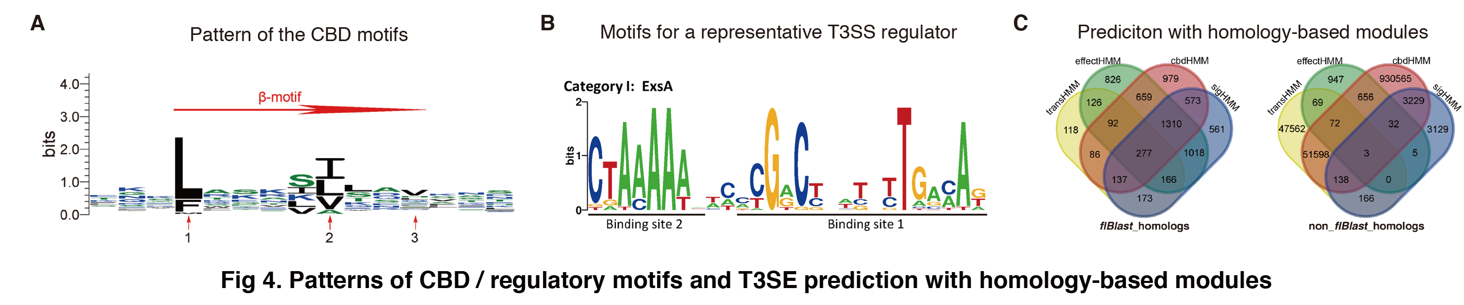
    (1) Methodology. The β-motif sequences reported by Lilic et al were downloaded and aligned with ClustalW using default parameters. HMMER 3.1 (hmmbuild) was used to build the HMM profile for the CBD motif sequences (Fig 4A). Targeted regions of candidate proteins were aligned to the profile and screened for the motifs with hmmsearch. Alternatively, a GO script using pattern recognition was also included in cdbHMM to find the conserved CBD motifs.

    (2) Optimized parameters and prediction. Intra-protein location analysis indicated that the β-motifs mainly started from N-terminal 21st ~90th amino acid of known effectors, and therefore only the N-terminal 100-aa peptide fragment of a candidate protein was extracted for β-motif screening. The similarity cutoff for prediction of CBD motifs with cbdHMM was set as the default cutoff E-value of hmmsearch.

7. Module 4: Prediction of Promoter Regulatory Motifs of Validated Effector Genes – transHMM

From an evolutionary point of view, a T3SE gene could potentially have co-evolved and been co-regulated with T3SS apparatus genes. Therefore, the promoters of T3SE genes from the same cluster of T3SSs could contain conserved motifs regulated by the pivotal T3SS regulators. The regulons of several key T3SS regulators were annotated and the motifs were identified as patterns for new effector gene scanning with transHMM.

7.1. Methodology of transHMM

Pivotal transcription regulators of T3SSs were annotated previously (Hu et al., 2017, Environ Microbiol, 19:3879-3895). The binding motifs within promoters of the regulated genes were annotated from literature (Fig 4B for an example). HMM profile was built for each regulator as done for sigHMM or effectHMM. To screen the motifs or patterns with transHMM, the 5’-upstream 2000-nucleotide sequence preceding the effector ORF was retrieved from each gene encoding the candidate protein, and the HMM profiles were screened one by one using hmmsearch with the default similarity cutoff E-value. Motif patterns were also screened with a pattern recognition method implemented in a GO script. The predictions with different homology-based modules were shown in Fig 4C.